Range
- 8.1~8.7
- 9.1~9.10
- 10.1~10.14
- 10.19~10.21
Chapter 8. Principal-Components Analysis
8.1. Introduction
Self-organized learning
- Self-organized learning is a type of unsupervised learning.
- locality of learning
8.2. Principles of Self-Organization
Principle 1: self-amplification
The following rule is based on Hebb’s postulate of learning.
- If two neurons of a synapse are activated simultaneously, then synaptic strength is selectively increased.
- If two neurons of a synapse are activated asynchronously, then?synaptic strength is selectively decreased.
Principle 2: competition
- The most vigorously growing synapses are selected.
Principle 3: cooperation
- Modifications in synaptic weights and neurons tend to cooperate with each other.
Principle 4: structural information
- The underlying structure in the input signal is acquired by a self-organizing system.
8.4. Principal-Components Analysis
Notations
- $m$: the dimension of the data space
- $l$: the dimension of principal components
- $\textbf{X}$
- $E[\textbf{X}]=\textbf{0}$
- Each row is a data vector.
- $\textbf{q}=\begin{bmatrix}q_1?& q_2 & … & q_m\end{bmatrix}^T$
- a unit vector that?$\textbf{X}$ is to be projected
- $A=\textbf{X}^T \textbf{q}=\textbf{q}^T?\textbf{X}$
- The projection of $\textbf{X}$ to $\textbf{p}$
- $\textbf{Q}=\begin{bmatrix}\textbf{q}_1 & \textbf{q}_2 & … & \textbf{q}_m\end{bmatrix}$
- $\textbf{R}$: the correlation matrix between?$\textbf{X}$ and?$\textbf{X}$
$E[A]=\textbf{q}^T E[\textbf{X}]=\textbf{0}$
8.5. Hebbian-Based Maximum Eigenfilter
Oja’s rule for maximum eigenfiltering
\[
w_{i}(n+1) = w_{i}(n) + \eta y(n)[x_{i}(n)-w_{i}(n)y(n)]
\]
\[i=1,2,…,m\]
- $w_{ji}(n)$: the synaptic weight from input unit $x_{i}(n)$ to output unit $y(n)$
- $m$: the number of input units
- $n$:?update step
- $\eta$: learning rate
- $||\textbf{w}(n)||^2=1$
- $\lim_{n\rightarrow \infty}{\sigma_{1}^{2}(n)}=\lambda_{1}$
- $\textbf{w}(n) \rightarrow \textbf{q}_1$ as?$n \rightarrow \infty$.?Then, $\textbf{q}_{1}$ are the principal component.

The Generalized Hebbian Algorithm (GHA)
\[
w_{ji}(n+1) = w_{ji}(n) + \eta y_{j}(n)[x_{i}(n)-\sum_{k=1}^{j}{w_{ki}(n)y_{k}(n)}]
\]
\[i=1,2,…,m, \ j=1,2,…,l\]
- $w_{ji}(n)$: the synaptic weight from input unit $x_{i}(n)$ to output unit $y_{j}(n)$
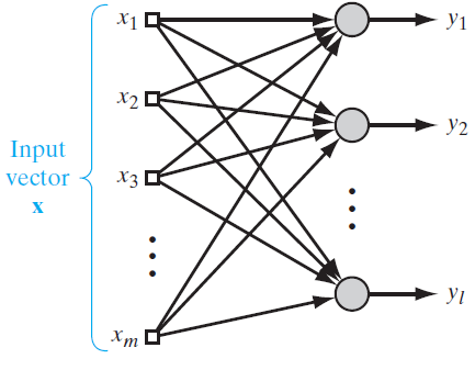
- $m$: the number of input units
- $l$: the number of output units
- $n$:?update step
- $\eta$: learning rate
- $||\textbf{w}_{j}(n)||^2=1$
- $\lim_{n\rightarrow \infty}{\sigma_{j}^{2}(n)}=\lambda_{j}$
- $\textbf{w}_{j}(n) \rightarrow \textbf{q}_{j}$ as $n \rightarrow \infty$. Then, $\textbf{q}_{j}$ are the principal components.
- a neural algorithm for PCA
Chapter 9. Self-Organizing Maps
9.1 Introduction
Self-organizing maps (SOMs)
A self-organizing map is a topological map of the input patterns.
The principal goal of the self-organizing map
- To transform an input pattern into a one- or two-dimensional discrete map
- To perform this transformation adaptively in a topologically ordered fashion.
9.3 Self-Organizing Map
SOM algorithm
- [Initialization] Initialize $\textbf{w}_{j}(0)$ and $n=0$
- [Sampling] Sample an input?\textbf{x}(n)
- [Similarity matching]?$i(\textbf{x}(n))\arg\min_{j}||\textbf{x}(n)-\textbf{w}_j||$
- [Updating] $\textbf{w}_j(n+1) = \textbf{w}_j(n) + \eta (n) h_{j, i(\textbf{x})}(n)(\textbf{x}(n)-\textbf{w}_{j}(n))$
9.4?Properties of the Feature Map
The four properties of the feature map
- Approximation of the input space
- The feature map, represented by the set of synaptic weight vectors, provides a good approximation to the input space.
- Topological ordering
- The feature map is topologically ordered in the sense that the spatial location in the output lattice corresponds to a particular feature of input patterns.
- Density matching
- Regions in the input space are mapped onto larger regions of the output space.
- Feature selection
- The SOM is able to select a set of best features for approximating the underlying distribution.
9.10 Relationship Between Kernel SOM and KL Divergence
Minimization of the KL divergence is equivalent to maximization of the joint entropy.
11.2?Statistical Mechanics
$p_i$: the probability of occurrence of state $i$
$E_i$: the energy of the system when it is in state $i$
$p_i$ if the system is in thermal equilibrium with its surrounding environment:
\[p_i=\frac{1}{Z}\exp(-\frac{E_i}{k_{B}T})\]
This probability distribution is called a Gibbs distribution or?Boltzmann distribution.
$T$: the absolute temperature in kelvins
- $T$ controls thermal fluctuations representing the effect of “synaptic noise” in a neuron.
$k_B$: Boltzmann’s constant
$Z$: a constant that is independent of all states
\[Z=\sum_{i}\exp(-\frac{E_{i}}{k_{B}T}})\]
But we use the following version without $k_{B}$ in machine learning.
\[p_i=\frac{1}{Z}\exp(-\frac{E_i}{T})\]
\[Z=\sum_{i}\exp(-\frac{E_{i}}{T}})\]
$F$: the Helmholtz free energy
\[F=-T\log(Z)\]
$<E>$: the average of the system
\[<E>=\sum_{i}{p_{i}E_{i}}\]
$<>$: the ensemble-average operation
\[<E>-F=-T\sum_{i}{p_{i}\log(p_{i})}\]
\[<E>-F=TH\]
because $H=-\sum_{i}{p_{i}\log(p_{i})}$
\[F=<E>-TH\]
$A$:the system we are interested in.
$A’$: the system that contact with $A$.
The total entropy of the?$A$ and $A’$?tends to increase. This can be denoted by $\Delta H + \Delta H’ \geq 0$.
The principle of minimal free energy
The free energy $F$ of the system tends to decrease and become a minimum in an equilibrium.
The resulting probability distribution is defined by the Gibbs distribution.
Nature likes to find a physical system with minimum free energy.
11.4 Metropolis Algorithm
- a?stochastic simulation?method
- a?stochastic algorithm for simulating the evolution of a physical system to thermal equilibrium
- a modified Monte Carlo method
- The Metropolis algorithm is commonly referred to as a Markov chain Monte Carlo (MCMC) method.
11.5. Simulated Annealing
- A stochastic optimization method
- annealing:?a process of heating and slow cooling in order to toughen and reduce brittleness.

Correspondence Between Statistical Physics and Combinatorial Optimization
11.6. Gibbs Sampling
- A stochastic simulation method
11.7. Boltzmann Machine
The Boltzmann machine is a stochastic binary machine that consists of stochastic neurons. A stochastic neuron resides in one of two possible states: +1 for the “on” state and -1 for the “off” state.
The stochastic neurons are partitioned into two groups: visible ones and hidden ones.
The visible neurons provide an interface between the network and the environment. The visible neurons are determined by the environment, which is a set of the input states.
The hidden neurons always operate freely. The hidden neurons are used to explain underlying constraints contained in the environmental input vectors. The hidden neurons capture high-order statistical correlations in the input states.
input pattern = input vector = a set of visible neurons = environment = environmental vectors
The primary goal of Boltzmann learning
The primary goal of Boltzmann learning is to produce a neural network that correctly models input vectors[patterns].
Pattern completion by the Boltzmann machine
The Boltzmann machine learns the correlations in the input vectors. Thus, when a input vector whose partial input states are unknown is given, the network is able to complete the unknown states.
Two assumptions in applying Boltzmann learning
- Each environmental input vector persists long enough to permit the network to reach thermal equilibrium.
- There is no sequential structure in the visible neurons.
Boltzmann learning
If it is possible to achieve such a perfect model, #(hidden units) is exponentially larger than #(visible units).
Two phases to the operation of the Boltzmann machine
- Positive phase: The network operates with environmental inputs[training samples].
- Negative phase: The network operates freely without no environmental inputs[training samples].
Boltzmann?machines
$\mathbf{x}$: the state vector of a Boltzmann machine
$\mathbf{x}_{\alpha}$: the state of the visible neurons. the realization of the random vector $\textbf{X}_{\alpha}$
$\mathbf{x}_{\beta}$: the state of the hidden neurons.?the realization of the random vector $\textbf{X}_{\beta}$
$w_{ji}$: the synaptic weight from $i$ to $j$ where $w_{ii}=0$ and?$w_{ji}=w_{ij}$
\[E(\textbf{x})=-\frac{1}{2}\sum_{i}\sum_{j\neq i}{w_{ji}x_{i}x_{j}}\]
\[(\textbf{X}=\mathbf{x})=\frac{1}{Z}\exp(-\frac{E(\textbf{x})}{T})\]
$P(\textbf{X}_{\alpha}=\mathbf{x}_{\alpha})$: the probability of the visible neurons in state?$\mathbf{x}_{\alpha}$
The objective of Boltzmann learning rule
To minimize the energy of the system given the training data $\mathfrak{T}$
To?maximize the probability of occurrence of state $i$
To maximize the log probability of occurrence of state $i$
Boltzmann learning rule
The probability of the visible?neurons
\[P(\mathbf{X}_{\alpha}=\mathbf{x}_{\alpha})=\frac{1}{Z}\sum_{\mathbf{x}=\mathbf{x}_{\beta}}{\exp(-\frac{E(\mathbf{x})}{T})}\]
\[Z=\sum_{\mathbf{x}}{\exp(-\frac{E(\mathbf{x})}{T})}\]
The overall probability distribution
\[P(\textbf{X}|\textbf{w})=\prod_{\textbf{x}_{\alpha}\in\mathfrak{T}}P(\textbf{X}_{\alpha}=\textbf{x}_{\alpha})\]
The overall log probability distribution
$L(\textbf{w})=\log\prod_{\textbf{x}_{\alpha}\in\mathfrak{T}}P(\textbf{X}_{\alpha}=\textbf{x}_{\alpha})$
$=\sum_{\textbf{x}_{\alpha}\in\mathfrak{T}}\log P(\textbf{X}_{\alpha}=\textbf{x}_{\alpha})$
$=\sum_{\textbf{x}_{\alpha}\in\mathfrak{T}}[\log \sum_{\mathbf{x}=\mathbf{x}_{\beta}(\textbf{x}_{\alpha})}{\exp(-\frac{E(\mathbf{x})}{T})} – \log \sum_{\mathbf{x}}{\exp(-\frac{E(\mathbf{x})}{T})}]$
The derivative of the overall log probability distribution
\[
\frac{\partial L(\textbf{w})}{\partial w_{ji}}=\frac{1}{T}\sum_{\textbf{x}_{\alpha}\in\mathfrak{T}}[\log \sum_{\mathbf{x}=\mathbf{x}_{\beta}(\textbf{x}_{\alpha})}{P(\mathbf{X}_{\beta}=\mathbf{x}_{\beta}|\mathbf{X}_{\alpha}=\mathbf{x}_{\alpha})}x_{j}x_{i} – \log \sum_{\mathbf{x}}{P(\mathbf{X}=\mathbf{x})x_{j}x_{i}}]
\]
where always $i\neq j$
11.9.?Deep Belief Nets
Training of a deep belief nets
- Training on a layer-by-layer basis
Chapter 12. Dynamic Programming
Key words
- Markov decision processes
- Bellman’s theory of dynamic programming
- policy iteration
- value iteration
- the direct learning-based approximation of dynamic programming
- temporal-difference learning
- Q-learning
- the indirect approximation of dynamic programming
- least squares policy evaluation
- approximate value iteration
Chapter 13.?Neurodynamics
Chapter 14. Bayesian Filtering for State Estimation of Dynamic Systems
Key words
- State estimation (theory)
- Dynamic systems
- State-space model
- State estimation of dynamic systems
- Kalman filters
- Bayesian filters
- Particle filters
14.1. Introduction
- Dynamic system
- Suppose there is a?sequence of times.
- At each time, there are a unknown state and the observation of the state.
14.2. State-Space Models
- Two components of the state-space model
- State model: $x_{n+1}=a_{n}(x_{n},w_{n})$
- Measurement[observation] model: $y_{n}=b_{n}(x_{n},v_{n})$
- $x_{n}$: state at time $n$
- $y_{n}$:?measurement at time $n$
- $w_{n}$: state noise at time $n$
- $v_{n}$: measurement?noise at time $n$
- Type 1: Linear, Gaussian state-space models
- State model / prediction: $x_{n+1}=A_{n+1,n}x_{n}+w_{n}$
- Measurement model / observation: $y_{n}=B_{n}x_{n}+v_{n}$
- $A_{n+1,n}$, $B_{n}$: linear transformations.
- $w_{n}$, $v_{n}$: zero-mean Gaussian distributions.
- Type 2: Nonlinear, Gaussian state-space models
- State model / prediction: $x_{n+1}=a_{n+1,n}(x_{n})+w_{n}$
- Measurement model / observation: $y_{n}=b_{n}(x_{n})+v_{n}$
- $a_{n+1,n}$, $b_{n}$: nonlinear transformations.
- $w_{n}$, $v_{n}$: zero-mean Gaussian distributions.
- Type 3: Linear, non-Gaussian models
- State model / prediction: $x_{n+1}=A_{n+1,n}x_{n}+w_{n}$
- Measurement model / observation: $y_{n}=B_{n}x_{n}+v_{n}$
- $A_{n+1,n}$, $B_{n}$: linear transformations.
- $w_{n}$, $v_{n}$:?non-Gaussian distributions.
- Type 4: Nonlinear, non-Gaussian models
- State model / prediction: $x_{n+1}=a_{n+1,n}(x_{n})+w_{n}$
- Measurement model / observation: $y_{n}=b_{n}(x_{n})+v_{n}$
- $a_{n+1,n}$, $b_{n}$: nonlinear transformations.
- $w_{n}$, $v_{n}$: non-Gaussian distributions.
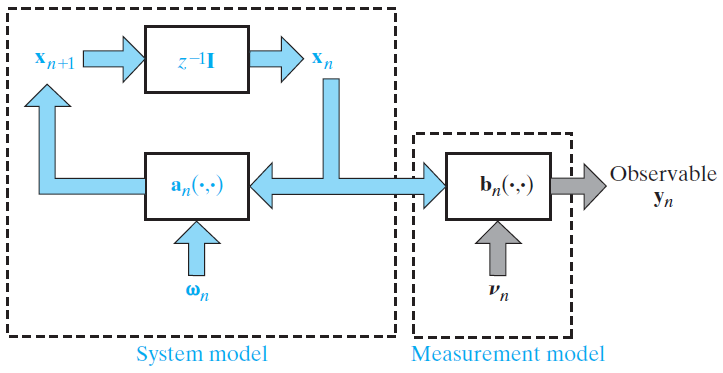
Figure 14.1 Generic state-space model of a time-varying, nonlinear dynamic system

Figure 14.2 Evolution of the state across time, viewed as a first-order Markov chain
14.3 Kalman Filters
- Kalman filters are linear, Gaussian state-space models.
- The parameters of Kalman filters
- $A_{n+1,n}$: The transition matrix
- $B_n$: The measurement matrix
- $w_n$: The Gaussian dynamic noise, which has zero mean
- $v_n$: The Gaussian measurement noise, which has zero mean
14.6 The Bayesian Filters
- A Bayesian filter is a method to solve the state estimation of a dynamic system.
- The Bayesian filter does not assume linearity and distributions of a space-state model.
- The only assumption of the Bayesian filter is that the evolution of the state is Markovian.
- The current state $x_n$ is only dependent on the previous state $x_{n-1}$.
- [?needed?]$l(y_1, …, y_n | x_1, …, x_n)=l(y_1|x_1)\cdot?… \cdot l(y_n|x_n)$
Update formula
1. Time update
\[
P(x_n|Y_{n-1})=\int{P(x_n|x_{n-1})P(x_{n-1}|Y_{n-1})dx_{n-1}}
\]
- $P(x_{n-1}|Y_{n-1})$ is given.
- ${P(x_n|x_{n-1})$ is solvable by $x_n=a_n(x_{n-1})$.
2. Measurement update
\[
P(x_n|Y_n)=\frac{1}{Z_n}P(y_n|x_n)P(x_n|Y_{n-1}) \ \textup{where} \ Z_n=P(y_n|Y_{n-1})
\]
- $P(y_n|x_n)$ is solvable by $y_n=b_n(x_n,v_n)$.
- $P(x_n|Y_{n-1}$ is given on the previous time update step.
- $Z_n$ is just a normalizing constant that ensures $P(x_n|Y_n)$ is probability between 0 and 1.
14.8 Particle Filters
- Particle filters are not just linear filtering but nonlinear filtering.
- A PF describe the indirect global approximation of the Bayesian filter.